Canonical correlation analysis (CCA) is a statistical technique that is used to understand the relationships between two sets of variables. It’s valuable in research contexts where understanding complex interrelations is key.
This section introduces the basic concept of CCA and a simple example of its application. The section also discusses the concept of standardisation, which is an important process to be applied to variables before embarking on CCA.
27.2 What is CCA?
Imagine you’re trying to understand the relationship between two ‘sets’ of things that you’ve measured.
For example, one set could be different aspects of students’ academic skills (like their reading, writing, and maths abilities), and the other set could be various lifestyle factors (like their hours of sleep, time spent on homework, and physical activity).
Canonical correlation helps to find out how these two sets of things are related to each other. It doesn’t just look at simple, one-on-one relationships (like reading ability -> hours of sleep). Instead, it tries to find the best possible combinations within each set that have the strongest link to each other.
So, in our example, canonical correlation would try to answer a question like: “Is there a combination of academic skills that is most strongly related to a certain combination of lifestyle factors?” Maybe it finds out that a mix of good reading and maths skills is most strongly linked to a combination of getting enough sleep and doing a moderate amount of homework.
Basically, canonical correlations are about finding the strongest possible connections between two sets of things, considering all the different ways they can be combined. It’s like looking for the best matching patterns between two complex puzzles.
27.3 The Purpose of CCA
Exploring relationships
As we’ve said, CCA investigates and quantifies the strength and nature of relationships between two sets ofvariables, where each set contains two or more variables.
CCA would help determine the degree to which these two sets of variables ‘move together’. We can then use these findings to predict one set of variables based on the other, or to understand the underlying structure between them.
Multivariate analysis
While simple correlation analysis provides a measure of the strength of the linear relationship between two individual variables, CCA is a multivariate technique that extends this concept to analyse the relationship between two sets of variables simultaneously.
This is particularly useful when the variables within each set are interrelated, which is often the case in real-world data (remember the concept of colinearity from earlier in the module).
CCA finds pairs of linear combinations (‘canonical variates’) from the variables of each dataset such that these pairs have the highest possible correlation with each other.
Important
It’s important to note that the relationships are between the sets of variables, not between individual pairs of variables.
This allows us to understand the multidimensional nature of the relationship between the sets, which is much richer and more informative than pairwise correlations.
27.4 Number of variables in each set
You might be wondering if we need to have the same number of variables in each dataset to conduct CCA.
The answer is no, it’s not necessary to have an equal number of variables in each set to perform CCA. CCA is designed to examine the relationships between two sets of variables, and these sets can have different numbers of variables.
However, there are some considerations to keep in mind:
The number of canonical correlations (the relationships between the sets) that can be examined is equal to the number of variables in the smaller set. For example, if you have 5 variables in one set and 3 in the other, you can only look at 3 pairs of canonical variables.
Having too many variables in relation to the number of observations can lead to overfitting and unstable estimates of the canonical correlations. This is a common concern in high-dimensional data scenarios.
It is essential to have a sufficient number of observations relative to the number of variables to ensure reliable results. As a rule of thumb, you want more observations than variables.
27.5 Steps in conducting CCA
Step One: Data preparation
As with all data analysis procedures, we need to ensure our data is correctly formatted, with two sets of variables ready for analysis.
Remember, CCA is based on examining the relationship between two sets of variables.
Standardisation
‘Standardisation’ is a fundamental concept step in data analysis. It’s used to ensure that each variable contributes equally to the analysis, and for facilitating comparison between different variables.
This is especially important when the variables are measured on different scales or have different units of measurement.
Without standardisation, a variable with a large range of values or higher magnitudes could disproportionately dominate the analysis, leading to biased results.
The basis of standardisation is transforming the data so that it has a mean of zero and a standard deviation of one. This process, known as z-score normalisation, allows for the comparison of scores from different distributions by converting them to a common scale.
The z-score is calculated by subtracting the mean of a variable from each observation and then dividing by the standard deviation.
This effectively ‘rescales’ the data to a standard normal distribution, which is a critical assumption in many statistical techniques, such as Canonical Correlation Analysis, regression models, and machine learning algorithms.
For now, we will not standardise our data before analysing it. We will use specific commands towards the end of our analysis to ensure that variability between how our different measurements have been conducted is accounted for.
However, you may find it helpful to explore how you (and when) you would go about standardising your data before analysis for the future…
Step Two: Exploring the data
We’re going to start by creating a data file which with 600 observations of seven variables.
Within this data file there are two different ‘sets’ of variables:
The first set, which might be called ‘psychological’ variables, are locus of control, self-concept and motivation.
There is a second set of ‘sport’ variables, which report performance in terms of speed, agility, endurance and strength.
This code generates the dataset data.
Show code
# Load necessary librarylibrary(MASS)# Set seed for reproducibilityset.seed(123)# Number of observationsn <-600# Means and standard deviations for all variables including 'motivation' as continuousmeans <-c(locus_of_control =0.0965333, self_concept =0.0049167, motivation =0.6608333, speed =51.90183, strength =52.38483, agility =51.849, endurance =51.76333)sds <-c(locus_of_control =0.6702799, self_concept =0.7055125, motivation =0.3427294, speed =10.10298, strength =9.726455, agility =9.414736, endurance =9.706179)# Define a covariance matrix with some arbitrary correlationscor_matrix <-matrix(c(1.00, 0.50, 0.30, 0.30, 0.60, 0.20, 0.60, # locus_of_control correlations0.50, 1.00, 0.25, 0.25, 0.55, 0.15, 0.75, # self_concept correlations0.30, 0.25, 1.00, 0.40, 0.60, 0.30, 0.50, # motivation correlations0.30, 0.25, 0.40, 1.00, 0.60, 0.40, 0.40, # speed correlations0.20, 0.15, 0.40, 0.60, 1.00, 0.45, 0.45, # strength correlations0.20, 0.15, 0.30, 0.40, 0.60, 1.00, 0.50, # agility correlations0.20, 0.15, 0.30, 0.40, 0.7, 0.50, 1.00# endurance correlations), 7, 7)# Convert correlation matrix to covariance matrixcov_matrix <-diag(sds) %*% cor_matrix %*%diag(sds)# Generate multivariate normal dataset.seed(123) # for reproducibilitydata <-mvrnorm(n, mu = means, Sigma = cov_matrix)# Convert to data frame and name columnsdata <-as.data.frame(data)names(data) <-c("locus_of_control", "self_concept", "motivation", "speed", "strength", "agility", "endurance")rm(cor_matrix, cov_matrix)
Our fundamental question in CCA is: is there a strong association between these two sets of variables? What is the direction of this association (positive or negative)? Do certain variables in each set contribute more strongly to this association than others?
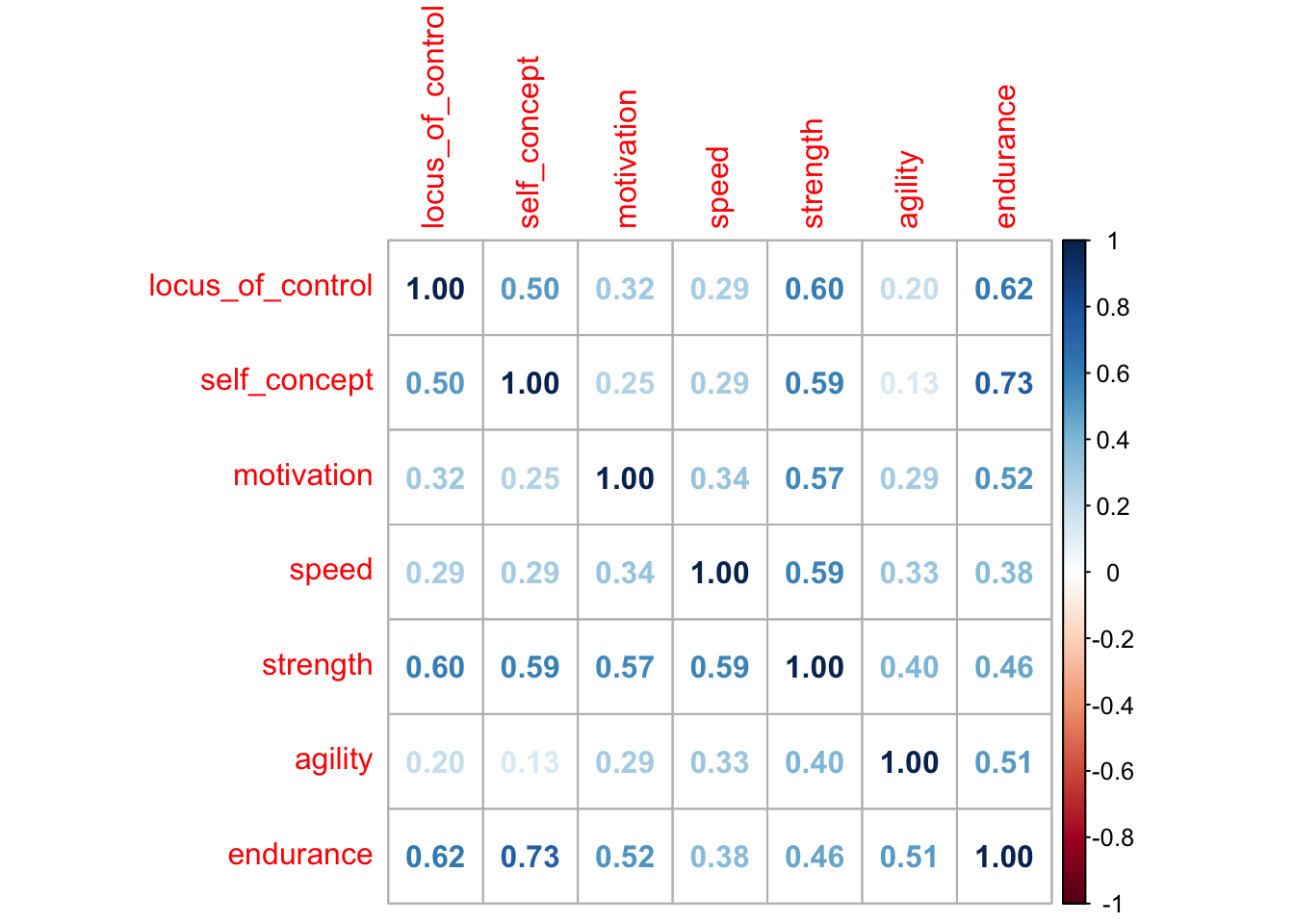
Let’s examine the correlation matrix between all our variables using the corplot package:
# Load the corrplot packagelibrary(corrplot)
corrplot 0.92 loaded
cor_matrix <-cor(data) # create the correlation matrixcov_matrix <-cov(data) # create the covariance matrix# Visualise correlation matrixcorrplot(cor_matrix, method ="number")
What’s the difference between a correlation matrix and a covariance matrix?
These are tools used in statistics to measure the relationship between variables, but they differ in how they express this relationship.
A covariance matrix represents the pairwise covariance between variables, indicating the direction and magnitude of the linear relationship between them. However, it does not provide information about the strength of this relationship on a standardized scale.
A correlation matrix, which arises from standardizing the covariance matrix, shows the linear relationship between variables in terms of correlation coefficients. These coefficients range from -1 to 1, providing a clear, dimensionless measure of how strongly two variables are related, regardless of their units of measurement.
The correlation matrix is more commonly used when the focus is on the strength and direction of relationships, rather than the magnitude of the variables involved.
From this, you can see that there are significant associations between some of the variables in the ‘psychological’ set and those in the ‘performance’ set (e.g. between locus of control and strength, and between self-concept and endurance).
So we good reason to suspect that our two sets of variables are associated with each other in a way that goes beyond chance.
Step Three: Conducting the CCA analysis
Now, I’m going to use the canon command to conduct the analysis.
First, I need to define which of my variables belongs to which ‘set’, and look at how the variables within each set are correlated with each other.
Next, we’ll look at the correlations within and between the two sets of variables using the matcor function from the CCA package (these will be similar to the results in our correlation matrix earlier).
Now, I can run the CCA analysis on our two sets of variables, using the cc command:
cc1 <-cc(psych, sport) # display the canonical correlationscc1$cor
[1] 0.99760742 0.25090395 0.06037605
What do these results tell us?
Canonical correlations quantify the overall association or relationship between the two sets of variables.
In other words, they tell you how strongly the linear combinations of variables in one set are related to the linear combinations in the other set.
In this case, the first canonical correlation is 0.998, indicating a strong and positive association between the two sets of variables (taken as a whole). It suggests there is a significant connection between the first canonical variates in each set (remember: this doesn’t refer to any specific variables).
The second canonical correlation is 0.322, which indicates that there a second positive association between the two sets of variables. It’s not as strong as the first canonical correlation.
There is a third, weaker canonical correlation of 0.147. Again, this suggests a positive association (higher psychological scores, higher performance scores).
Three canonical correlations have been produced because the smallest number of variables in one of the sets is three.
Interpretation of canonical correlations can be challenging because they represent relationships between linear combinations of variables rather than between individual variables.
Now, I’m going to examine the raw canonical coefficents:
These canonical coefficients give important clues as to the relationship between our two sets of variables.
They tell us how much each variable (like locus of control, or strength) contributes to the relationship that was found for each canonical correlation (1, 2 and 3).
Higher coefficients mean that the variable is more important in linking the two sets of data.
I’m going to stick with the first canonical correlation that we found (0.998).
In the example above, the numbers for the first canonical relationship for our psychological variables are -0.50 (locus of control), -0.85 (self concept), -1.08 (motivation).
The larger the absolute value of a coefficient (regardless of whether it’s positive or negative), the more significant the role of that variable in the relationship.
This means:
-1.08 has a greater absolute value than -0.85, so motivation plays a more significant role in the relationship compared to self_concept.
The sign (+ or -) indicates the direction of the relationship. A positive coefficient (like 0.017 or 0.04) suggests that as the value of this variable increases, the related variable in the other set tends to increase. A negative coefficient (like -0.07 or -0.08) indicates the opposite: as the value of this variable increases, the related variable tends to decrease.
Compare the coefficients to each other. In the coefficients for the sport variables, -0.08 is the largest in absolute terms, suggesting endurance has the strongest individual influence.
Next, we’ll use comput to compute the loadings of the variables on the canonical dimensions (variates). These loadings are correlations between variables and the canonical variates.
These correlations are between observed variables (the variables we measured) and canonical variables which are known as the canonical loadings.
These are what we initially observed as our canonical correlations (0.998, 0.322, 0.147).
These canonical variates are actually a type of latent variable.
Just like raw canonical coefficients, the relative magnitude (ignoring + and -) of the loading (how big or small the number is) is important. Larger absolute values mean the variable is more closely related to the canonical variable.
For statistical tests, we use R package “CCP”.
# tests of canonical dimensionsrho <- cc1$cor## Define number of observations, number of variables in first set, and number of variables in the second set.n <-dim(psych)[1]p <-length(psych)q <-length(sport)## Calculate p-values using the F-approximations of different test statistics:p.asym(rho, n, p, q, tstat ="Wilks")
Wilks' Lambda, using F-approximation (Rao's F):
                stat     approx df1      df2      p.value
1 to 3:  0.004462226 880.552831  12 1569.222 0.000000e+00
2 to 3:  0.933631420   6.916751   6 1188.000 3.084748e-07
3 to 3:  0.996354733   1.088435   2  595.000 3.374127e-01
The first test of the canonical dimensions tests whether all three dimensions are significant (they are, F = 880.55), the next test tests whether dimensions 2 and 3 combined are significant (they are, F = 6.92). Finally, the last test tests whether dimension 3, by itself, is significant (it is). Therefore dimensions 1, 2 and 3 are each significant.
When the variables in our model have very different standard deviations, the standardised coefficients allow for easier comparisons among the variables. Next, we’ll compute the standardised canonical coefficients.
The standardised canonical coefficients are interpreted in a manner analogous to interpreting standardised regression coefficients. For example, consider the variable speed, a one standard deviation increase in reading leads to a 0.17 standard deviation decrease in the score on the first canonical variate for set 2 when the other variables in the model are held constant.
27.6 Conclusion
There has been a lot of ground to cover in this section!
Don’t worry if it hasn’t all made sense; we’ll return to it in detail during this week’s practical session.